Filters are the algorithms use to
find the state of a system. A system can be a robot moving in a known or
unknown environment and the state at any given time instance could be its position coordinates or velocity. Bayesian Filter, as the name signifies, is a recursive state estimation technique and is used when the state
of the system is held constant.
Before moving further lets discuss about two types of probabilities:
- Bayesian or Personal. The Bayesian probability of an event is a person’s degree of belief in that event. It is the property of the person who assigns that probability. For example, if somebody asks two persons, what is the probability that India will win a cricket match against Pakistan? Then one might reply 0.9, while other might say 0.2. The numbers 0.9 and 0.2 represents the degree of belief of each person and this varies from person to person. Statisticians who follow this definition are known as Bayesians.
- Physical Probability. This probability is the actual physical probability of an event. For example, the probability of getting a head after tossing a coin. This probability is calculated by repeating the experiment a favorable number of time. In the above example we can repeat the experiment by tossing the coin 1000 times and reporting the number of heads. Statisticians who follow this definition are known as Frequentists.
Now lets move forward and have a look at Bayes’ theorem which is the key concept in Bayesian filters and is given by:
$\ P(H|D) = $ $\frac{P(D|H)P(H)}{P(D)}$
Here \(\ H\) is our hypothesis and \(\ D\) is
the observed data.
\(\ P(H|D)\) is called the posterior belief i.e. the probability
after observing data \(\ D\).
\(\ P(H)\) is called the prior belief about the hypothesis \(\ H\).
\(\ P(D|H)\) is called the likelihood of data \(\ D\) given the particular hypothesis \(\ H\).
\(\ P(D)\) is the normalizing constant to make \(\ P(H|D)\) a distribution and is given by $\int P(H)P(D|H)~dH$.
Bayesian filter is the most
general algorithm to calculate beliefs given some data. After the observation of data $\ D$ it has two steps:
- For each possible value of hypothesis calculate the un-normalized belief given by $\ P(D|H)P(H)$ . Prediction and innovation
- Then normalize the un-normalized belief by dividing it by $\int P(H)P(D|H)~dH$.
After performing these two steps update $\ P(H) = P(H|D)$ and then repeat the above two steps again till we are pretty much sure about the degree of belief about the hypothesis $\ H$.
Example:
The example is adapted from
Prof. Michael A. Goodrich
Let us assume that we have a
system in a two dimensional space and the true state of the system is $\ S = (3, 5)$.
But the true state is unknown to us and we want to estimate it. For simplicity let’s
assume that the world is discrete and have 9 possible states, but we can have finer
grids than this.
$\ (2, 4)
(3, 4) (4, 4)$
$\ (2, 5) (3, 5) (4, 5)$
$\ (2, 6) (3, 6) (4, 6)$
$\ (2, 5) (3, 5) (4, 5)$
$\ (2, 6) (3, 6) (4, 6)$
Suppose we have some kind of sensor that gives
us the measurements about the true state, but the sensor is noisy. So our
measurement is $\ X = S + \eta$ where $\ S$ is the true state and $\eta$ is the noise. Let’s
assume that the noise is Gaussian with $\mu = 0$ and variance $\sigma^2$.
Let’s assume that initially we
are completely uncertain about the state of the system so we assign uniform
probability to each possible state. So our prior distribution $\ P(S) = 1/9$. Now
we have to calculate the likelihood $\ P(X|S)$. Recall that noise $\eta$ is Gaussian and $\ X = S + \eta$ , so if we know $\ S$ this implies that $\ X$ is also Gaussian. To calculate
the mean value of$\ X$ we can use the principle of linearity for expectation.
$\ E(X) = E(S) + E(\eta) = S + 0 = S$ as
$\ S$ is known so it’s a constant and mean
for $\eta$ is 0.
So $\ P(X|S)$ is Gaussian with mean $\ S$
and variance $\sigma^2$. Therefore $\ P(X|S)$ is given by:
$\ P(X|S) = $ $\frac{1}{\sigma \sqrt{2\pi}} e^{-(X - S)^2 / 2\sigma^2}$
The only unknown left term is $\ P(X)$
which is given by $\sum\limits_{S} P(S)P(X|S)$. So $\ P(S|X)$ is given by:
$\ P(S|X) = $ $\frac{P(X|S)P(S)}{P(X)}$
We repeat the above procedure for
each measurement till we are pretty much sure about the degree of belief about
the true state $\ S = (3, 6)$. The easiest way to do this is to set $\ P(S) = P(S|X)$
and then repeat for another data point $\ X$.
Figures and Code:
Code can be downloaded from my github account.
Sampling of 100 points with standard deviation of 2. Red point is the true state of our system $\ S = (3, 5)$
Figures and Code:
Code can be downloaded from my github account.
Sampling of 100 points with standard deviation of 2. Red point is the true state of our system $\ S = (3, 5)$
Convergence to true position and posterior distribution:
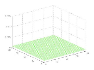
Initially posterior is uniform due to the state of total confusion:
After 20 iterations:
After 50 iterations:
After 100 iterations:
The last figure shows that our belief about the true state has converged to $\ (3, 5)$


